Features Selection in the Age of Generative AI
By QTS Capital Management LLC Prepared by Ernest Chan, Chairman, and Nahid Jetha, CEO

Features are inputs to machine learning algorithms. Sometimes also called independent variables, covariates, or just X, they can be used for supervised or unsupervised learning, or for optimization. For example, at QTS, we use more than 100 of them as inputs to dynamically calibrate the allocation between our Tail Reaper strategy and E-mini S&P 500 futures. In general, modelers have no idea which features are useful a priori, or if they are redundant, for a particular application. Using all of the features can result in overfitting and poor out-of-sample performance, or worse, numerical instability and singularities during matrix inversion. Hence the need for a process called “features selection”.
In conventional, “discriminative” AI, we try to model the probability P(Y|X), where Y is variously called the dependent variable, the target, the label, or the variate. Quant traders often use tree-based models such as gradient-boosted trees (GBT), and features selection algorithms such as MDA, SHAP, LIME are often used to select a subset of features that are useful for modeling P(Y|X). In Generative AI (GenAI), features adopt a much more central role than the target variable. Complicated deep neural networks (DNN) are built just for modeling the probability distribution of X, regardless of what Y they may be used to predict. Often, we pre-train one DNN with one objective (such as how well it models the distribution of X), and use it for another objective (such as optimizing some reward using deep reinforcement learning). We can no longer use MDA, SHAP, or LIME in cases where Y isn’t yet defined. But more importantly, such conventional features selection techniques are global: they do not allow for sample-specific features selection. Once a subset of features is selected, it is used for every inference, which limits the model’s adaptability and flexibility. Here we will discuss two powerful and well-known methodologies in deep learning / Generative AI that can be used for features selection: the transformer, and the variational autoencoder. They can be used to pre-train a DNN for different downstream applications or with a large set of unlabeled data, they allow for sample-specific features selection, and they can be trained jointly with the DNN parameters using a single objective function.
I discussed how transformers are constructed in a series of blog posts here, here, and here. In self-attention transformers, the sum of attention scores in a column of the attention matrix gives the feature importance scores of a feature corresponding to that column. If we multiply the attention matrix with the input features (or some linearly transformed version of them), we get the “context vector” Z, which is our transformed feature vector with each feature weighted by their importance (attention) score. Note these attention scores depend on the features’ values themselves, so they are sample-specific. The way to train the parameters of a transformer is to use it to achieve some objective, such as maximizing the log likelihood of a classification task. One can also pre-train a transformer in an unsupervised setting (i.e. without labels): simply use Z to reconstruct (instead of predict) the original features, using Mean Squared Error (MSE) as the loss function. But once trained, the transformer can be used unmodified for other downstream tasks such as regression or optimization. We can also choose to fine-tune it by adapting its parameters (hopefully just slightly) to optimize other objectives. This pre-training and fine-tuning paradigm is one reason why GenAI is so powerful compared to traditional discriminative AI: we can pre-train a GenAI model on a much larger set of (possibly unlabeled) data that are related to the one we are trying to predict. For example, if we are creating features to predict the returns of AAPL, we could pre-train the transformer on features from MSFT, GOOG, etc. first, then fine-tune the parameters to predict AAPL’s returns (see section 10.5 of our book on fine-tuning.) This potentially allows us to overcome the perennial data scarcity problem in financial machine learning.
Beyond these delightful advantages of using transformers for feature selection, cross-attention transformers also allow us to mix time-series (e.g. VIX, interest rate, HML factor, ...) and cross-sectional (i.e. stock-specific e.g. P/E, B/M, Dividend Yield, ...) features together, or to mix cross-sectional features from different instruments (e.g. NVDA, GOOG, ...). (See our blog post for the difference between time-series and cross-sectional features.)
If one were to use cross-sectional features as “query”, and time-series features as “key/value” in a cross-attention transformer, then the sum of the attention scores in a column represent the importance of a time-series feature across all cross-sectional features in predicting, for example, that stock’s returns. The context vector Z has the same number of rows as the number of cross-sectional features, but they are modulated by the time-series features at that snapshot in time. This is a graceful way to apply macro-economic context to stock-specific fundamentals.
Let’s look at an example for predicting SPX returns. Suppose we simply buy-and-hold SPX - an impossibility, since it’s an index rather than an ETF, but this is just for illustration. (In the same spirit, we’ll ignore transaction costs in all examples.) The SPX has a Sharpe ratio of 0.39 over 2005-2017, and 0.8 over 2017-2025. We’ll designate the first period as the train set and the second as the test set for the following ML tasks. Using 14 technical features created using TA-LIB library, we train a simple MLP neural net with 1 hidden layer and 2 hidden nodes per layer to predict its next-day return and go long if the predicted return is positive and hold cash otherwise. The Sharpe is (0.4, 1.1) on the (train, test) sets. The MLP outperforms buy-and-hold. If we create a self-attention transformer with 64-dimensional “embedding” for the features and proper normalization, while also adding lagged features with lags of 1, 2, 3, and 4 days, and feed the context vector into the same MLP, then the Sharpe becomes (0.7, 0.6). It still outperforms buy-and-hold, but it doesn’t perform as well as the MLP with the original, un-transformed, features. This holds a lesson - transformers sound wonderful, but without enough data, overfitting is a real danger. There are also many hyperparameters that we can optimize for a transformer, such as the embedding dimension, the normalization method, the number of attention heads, adding positional encoding, etc. You can read all about these variations in my previously cited blog posts. If we add just VIX as the time-series feature to be used as the key/value input, a cross-attention transformer will give us Sharpe of (0.3, 0.6). No improvement. But of course, this is a toy example. In practice, we should use the hundreds of time-series features (including both macro-economic and market-based features) that QTS and Predictnow.ai jointly created as key/value input. (The performance examples shown are hypothetical and for illustrative purposes only. No representation is being made that any account will or is likely to achieve profits or losses similar to those shown. Past performance is not necessarily indicative of future results. Full hypothetical disclaimer below.)
Variational autoencoder (VAE) is the other method of features selection. It can also be thought of as a more general version of the familiar PCA, Gaussian Mixture Model (GMM), or Hidden Markov Model (HMM). All these are latent variable models that convert the observable features X into a smaller set of unobservable, “latent”, variables z that can generate the observable features with simpler probability distributions (such as Gaussian.) In other words, if z is the latent variable, which could be as simple as a binary categorical variable z=(0, 1) with Bernoulli distribution or a continuous variable with Gaussian distribution, then
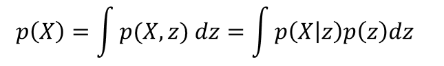
This is also reminiscent of the context vector Z from the transformer output. In both cases, z tells you the probability distribution of the ultimate output of the AI system. In the VAE case, we have an unsupervised learning task, so the output is the same as the input X. Given z, we obtain X via P(X|z): that’s called the decoder part of a VAE. But how do we get the distribution of z given X? Finding p(z|X) is the encoder’s job. Both p(X|z) and p(z|X) are Gaussians, but their parameters are given by two separate DNNs. Combining the two DNNs constitute the VAE, and the two sets of parameters are trained simultaneously by minimizing the log likelihood of X. This is easier said than done, but details can be found in Chapter 6 of our book. I will also dive deeper into VAE in my workshop at Imperial College London, and will elaborate on the relationship among GMM, HMM, and VAE, and their training methodologies in a future blog post.
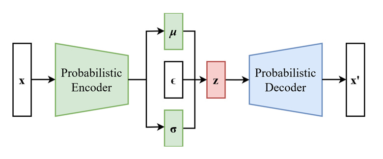
Source: https://en.wikipedia.org/wiki/Variational_autoencoder#/media/File:Reparameterized_Variational_Autoencoder.png
(If you’re wondering, we also need to specify the prior p(z), which is usually assumed to be a simple fixed Gaussian, p(z)=(0, I).)
Once trained in this unsupervised manner, the latent variable z can be used as a converted feature vector for downstream supervised learning or optimization applications, much like the context vector Z from a transformer. In fact, the transformer can be thought of as an encoder. Also, similar to the transformer, we can pre-train the encoder with one large unlabeled data set, and fine-tune it on a small labeled data set for supervised learning. Alternatively, we can apply “semi-supervised” learning (Kingma and Welling 2019) where a mixture of unlabeled and labeled data is used to train the VAE. When semi-supervised learning was applied to image classification, just 10 labels per class were needed to achieve a >99% classification accuracy. Amazing! This holds great potential for many applications with limited labeled training data.
Continuing on the next-day SPX return prediction example above, we can build a VAE using the same 14-dimensional feature vector, a 8-dimensional latent vector, and 2 ReLU layers each for the encoder and decoder. The Sharpe is (0.2, 0.4) on the (train, test) sets, which is quite a bit worse than the buy-and-hold benchmark. Naturally, significant hyperparameter and architectural optimization needs to be done. More importantly, we haven’t pre-trained the VAE on any extra data, so it isn’t surprising that the SPX data itself is insufficient to produce good performance.
Transformers and Variational Autoencoders illustrate how feature transformation and selection are central to GenAI, rather than an afterthought, as in traditional discriminative models. They also highlight the flexibility of generative approaches, particularly the ability to pre-train models on large unlabeled datasets and fine-tune them incrementally as new data becomes available. Their potential in financial applications is just now being exploited by some of the most sophisticated quantitative trading groups.
===
To learn more about GenAI, join me at Imperial College London for a weekend workshop on Trading with GenAI, Nov 22-23, 2025. Register at https://www.meetup.com/thalesians/events/311100776
DISCLAIMER:
QTS Capital Management LLC (“QTS”) is a Commodity Trading Advisor and Commodity Pool Operator registered with the U.S. Commodity Futures Trading Commission and a Member of the National Futures Association.
This material is provided for educational and informational purposes only and does not constitute investment advice or an offer to buy or sell any financial instrument.
Performance examples shown are hypothetical and for illustrative purposes only. No representation is being made that any account will or is likely to achieve profits or losses similar to those shown. Past performance is not necessarily indicative of future results.
All investments involve risk, including the possible loss of principal. There can be no assurance that an investment strategy will achieve its objectives or will otherwise meet expectations. Futures trading is not suitable for all investors.
Hypothetical performance results have many inherent limitations, some of which are described below. No representation is being made that any account will or is likely to achieve profits or losses similar to those shown. In fact, there are frequently sharp differences between hypothetical performance results and the actual results subsequently achieved by any particular trading program. One of the limitations of hypothetical performance results is that they are generally prepared with the benefit of hindsight. In addition, hypothetical trading does not involve financial risk, and no hypothetical trading record can completely account for the impact of financial risk in actual trading. For example, the ability to withstand losses or to adhere to a particular trading program in spite of trading losses are material points which can also adversely affect actual trading results. There are numerous other factors related to the markets in general or to the implementation of any specific trading program which cannot be fully accounted for in the preparation of hypothetical performance results and all of which can adversely affect actual trading results.