Deep Reinforcement Learning for Portfolio Optimization
Is it really better than PredictNow.ai's Conditional Portfolio Optimization scheme?


We wrote a lot about transformers in the last three blog posts. Their sole purpose was for feature transformation / importance weighting. These transformed and attention-weighted features will be used as input to downstream applications. In this blog post, we will discuss one such application: portfolio optimization via deep reinforcement learning. We will based our example on a paper by Sood et. al. (2023) Ref. [1] (see references at the end.)
In supervised learning, we want to predict a label (target ) using a set of features (predictors), and we train an ML model using many samples of (features, label) pairs. In reinforcement learning (RL), we want to maximize an objective using a sequence of actions (hence this is sometimes called “sequential decision making”). Each action a(t) at time t is based on the state variables s(t) at time t, and the next state s(t+1) may (but not necessarily) depend on s(t) and a(t). Note that in general both a and s can be vectors or even matrices. The state variables in RL correspond to the features in supervised learning. After an action a(t) is taken, we receive a reward r(t), a scalar. In the simplest case (such as the example we are considering), the ultimate objective is to maximize the expected total reward J=E[r(0) + r(1) + … + r(T)], assuming that we have a fixed time horizon that terminates at T. (If there is no terminal time, we apply a discount factor to each future reward to reduce its contribution, so that the total sum doesn’t go to infinity, but this doesn’t concern us in practical usage since we always train with finite data.) The ML model inside deep reinforcement learning (DRL) is used to learn from a sequence of (s(t), a(t), r(t)) for t=0, 1, 2, … to generate the optimal a(t) given an input s(t), with the goal to maximize J. People call this ML model a policy π. It is important to note that π is a probability distribution over actions conditioned on states, π( a(t) | s(t) ). The action is not a deterministic function of the state. That’s why the objective of DRL is to maximize expected total reward and not the realized total reward from one sample sequence of (s(t), a(t), r(t)). In fact, even the sequence of states aren’t usually deterministic: s(t+1) could be a probabilistic function of s(t) and a(t). Using these symbols, we can state the RL problem more succinctly as
where ~ denotes that the action at is sampled from a probability distribution π(a(t)|s(t)). See Ref. [2] for more details. We have used st and at to denote s(t) and a(t) for notational simplicity.
Usually we parametrize the policy function / conditional probability distribution π by a parameter θ, which may represent the mean and variance of a Gaussian, the most common assumed distribution. So equation (1) becomes
Let’s consider how all this work in the portfolio optimization example in Ref. [1]. The portfolio composes of the 11 SPX sector subindices plus cash.
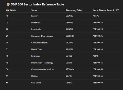
The state variables are the % allocations in the portfolio just prior to the reallocation actions, lagged log returns of each of these subindices over 60 days, the VIX, and historical volatility of SPX over a couple of lookback periods. We can of course include the features that we obtained from the transformer described in the previous blog post as state variables too. The action variables are the % capital allocation to the 11 SPX sector subindices and cash. The constraint on these actions is that these 12 actions must sum to 1, and each of them must be positive as we have a long-only portfolio. (However, since the 12th action is the cash weight, this means the portfolio can be all cash only.) This implies that the portfolio is rebalanced to a gross market value of 1 at each time step. All these are easy to understand. The reward rt, however, requires some thought. Typically, we optimize a portfolio to achieve the highest Sharpe ratio (that is called the “tangency portfolio” in the Markowitz mean-variance optimization) from t=1 to t=T. However, in RL we need to have instant gratification, i.e. we need an immediate reward in response to an action-state pair in order to make incremental update to the policy π (typically a neural net in DRL). We cannot take a random sequence of actions and see what the Sharpe ratio at time T is, otherwise there is no “reinforcement” to speak of. On the other hand, we cannot just set rt to the next-day return R(t+1), because that would obviously result in the objective function becoming the arithmetic return. (Note we use uppercase R to represent financial return, and lower case r to represent RL reward.) What can we sum that will result in a Sharpe ratio? Why, the differential Sharpe ratio, of course.
The differential Sharpe ratio D(t) is defined as the change of the Sharpe ratio per unit time. More specifically, it tells us how much the Sharpe ratio changes at time t because the portfolio returned R(t). It is not very illuminating to look at its exact algebraic form (which is displayed in Ref. [1]). Suffice it to say that it is a simple function of all the past returns R(1), R(2), …, R(t).
Now that we have all the elements of the RL setup, all that is left is to choose the specific RL algorithm. The paper picked Proximal Policy Optimization (PPO), invented by OpenAI, which is a conventional choice. As with all things neural-net, one uses gradient ascent (descent) to maximize (minimize) a reward (cost) function, so we shall update θ in equation (2) by
where α is the learning rate. So how do we compute the gradient? π(a|s) is represented by a neural network (as we shall see, a two-layer MLP) and is differentiable. Its gradient can be computed by the usual backpropagation technique (see Chapter 3 of our book). However, there is no analytical function that relates π and J, as the expectation is not only over the different actions that π might take for a given state, but also over the different states that may result from previous actions (though in our portfolio optimization example, the states aren’t dependent on previous actions). Fortunately, the famous REINFORCE algorithm (also discussed in our book in another context) comes to the rescue: the gradient of the expectation of J is equal to the expectation of the gradient of log π, weighted by the cumulative forward reward of the trajectory:
Note that the inner sum represents the cumulative reward from t to the terminal time T. We can simulate a trajectory (sequence) of (s, a, r), use these to compute the gradient of the log of the policy function via backprop, and obtain the value inside the expectation [.] in equation (4). We can get a better estimate of the expectation value if we average this value at each time step t over multiple trajectories. (See Algorithm 1 in Ref. [2]).
At this point, it is worthwhile to clear up some confusion about online vs offline RL. As you can see from equation (4), during the training phase to find the optimal θ, we need access to the entire historical trajectory (sequence) from t=0 to T. You may think this is “offline” RL since we are not updating the policy π as we move forward in real-time one time step at a time. But no, this is still “online” RL, as we are able to simulate rt in response to any at and st. In a true “offline” RL, we would have one fixed historical trajectory (the actual trajectory taken) and no “counterfactual” - i.e. we wouldn’t know rt+1 and st+1 in response to a different action at. (An example of an offline RL is to optimize consumer product prices based on how demand is affected if prices are changed. Nobody knows what that historical counterfactual demand would have been.) Since financial optimization usually depends only on market prices, there is no difficulty in simulating the what-if scenario (“What if we allocate more money to NVDA instead of TSLA?”), so financial RL is almost always online RL.
You may think that since equation (4) details how we can train and optimize the policy π, our optimization problem is solved. However, there remains a practical problem with estimating the expectation in equation (4): the well-known “high variance” problem in DRL. To wit, since the policy function produces a different action sampled from a probability distribution at each time step, there are lots of randomness in the trajectories used in estimating the expectation. We may need an impractically large number of trajectories to overcome this randomness / variance via the law of large numbers. One quick fix to this is to subtract the “baseline” reward b from the reward (.) inside equation (4), i.e. we weigh a trajectory only based on its outperformance from the baseline performance. The mathematical idea behind it is very simple: if you subtract a random variable Y from a random variable X where Y has zero mean, you can adjust Y so that the variance of X-Y has lower variance than X but has the same mean (expectation value). For details, see this excellent blog post (Ref.[5]). With this trick, equation (4) can be rewritten
where we abbreviated the cumulative reward from t to T as ℛₜ , and the baseline reward as b(st) which indicates it depends on the state st. We can interpret b(st) as the expected “value” (i.e. expected forward cumulative reward) of the state st from t to T. This interpretation leads us to the next method of variance reduction: we can train a separate RL model to predict the value of a state. This RL model is called the “critic”, and ℛₜ-b(st) is replaced by the general function called “advantage” A(st, at). “Advantage” describes the outperformance of a proposed action over some baseline or average or expected reward. As you can see, A is a function of both the state and the action at time t, which resembles the Q function of Q-learning, which is a traditional RL learning algorithm. There are at least 3 ways to compute the advantage A, all detailed in the blog post quoted above. The one chosen for the portfolio optimization problem is Generalized Advantage Estimate (GAE), see Ref. [1]. In general, these methods are called Advantage Actor Critic (A2C) in DRL. So equation (5) can be rewritten as
The final step in improving the stability of training a policy is to avoid policy updates that are too large. Quoting Ref. [3]: “To do that, we use a ratio that indicates the difference between our current and old policy and clip this ratio to a specific range[1−ϵ, 1+ϵ].” Equation (6) becomes
where
with
Now back to the portfolio optimization example. The paper trains 5 separate “agents” in parallel over a 5 year training window. To paraphrase this: we run 5 independent simulations of 5 year training window and compute 5 independent policies. We then pick the agent (i.e. policy) that performed best in the next 1 year validation window to be used as the seed policy for the next training window (which is the old window rolled forward by one year). For the 1-year out-of-sample period that immediately follows the validation window, we create 5 portfolios due to the 5 independent policies and obtain their average returns and compute other performance metrics on these returns.
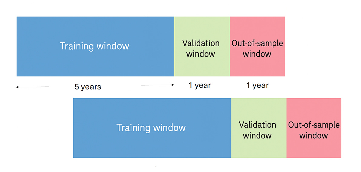
The training for each agent/ policy consists of gradient updates based on equation (7) but over 10 trajectories (“environments”) in parallel, each trajectory going from the beginning to the end of each training window 600 times (600 × 5 × 252 = 600 × 1,260 trading days). That’s easy to accomplish because we can simply take the average of the summand over different trajectories in each time step in equation (7). The gradient update occurs once after every 3 years during the 600 cycles, so T=756.
The policy function is represented by a two-layer [64, 64] MLP with tanh activations.
Ernie’s team at Predictnow.ai implemented this DRL strategy, and compare that with other conventional portfolio optimization methods, including PredictNow.ai's proprietary Conditional Portfolio Optimization (CPO) method (Ref. [7]), which is far simpler than DRL. Here are the results:
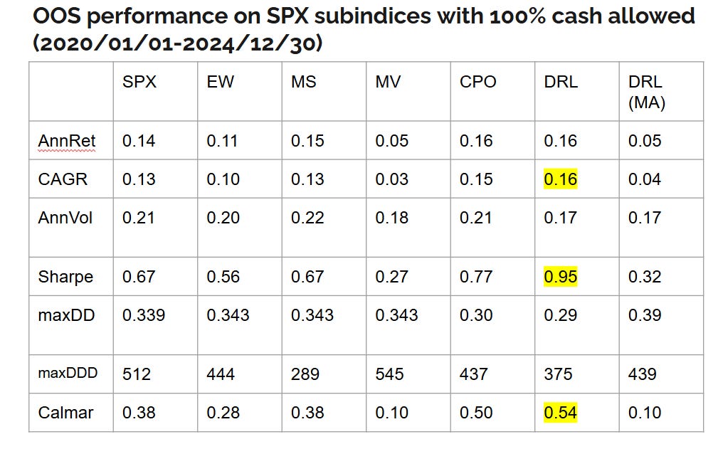
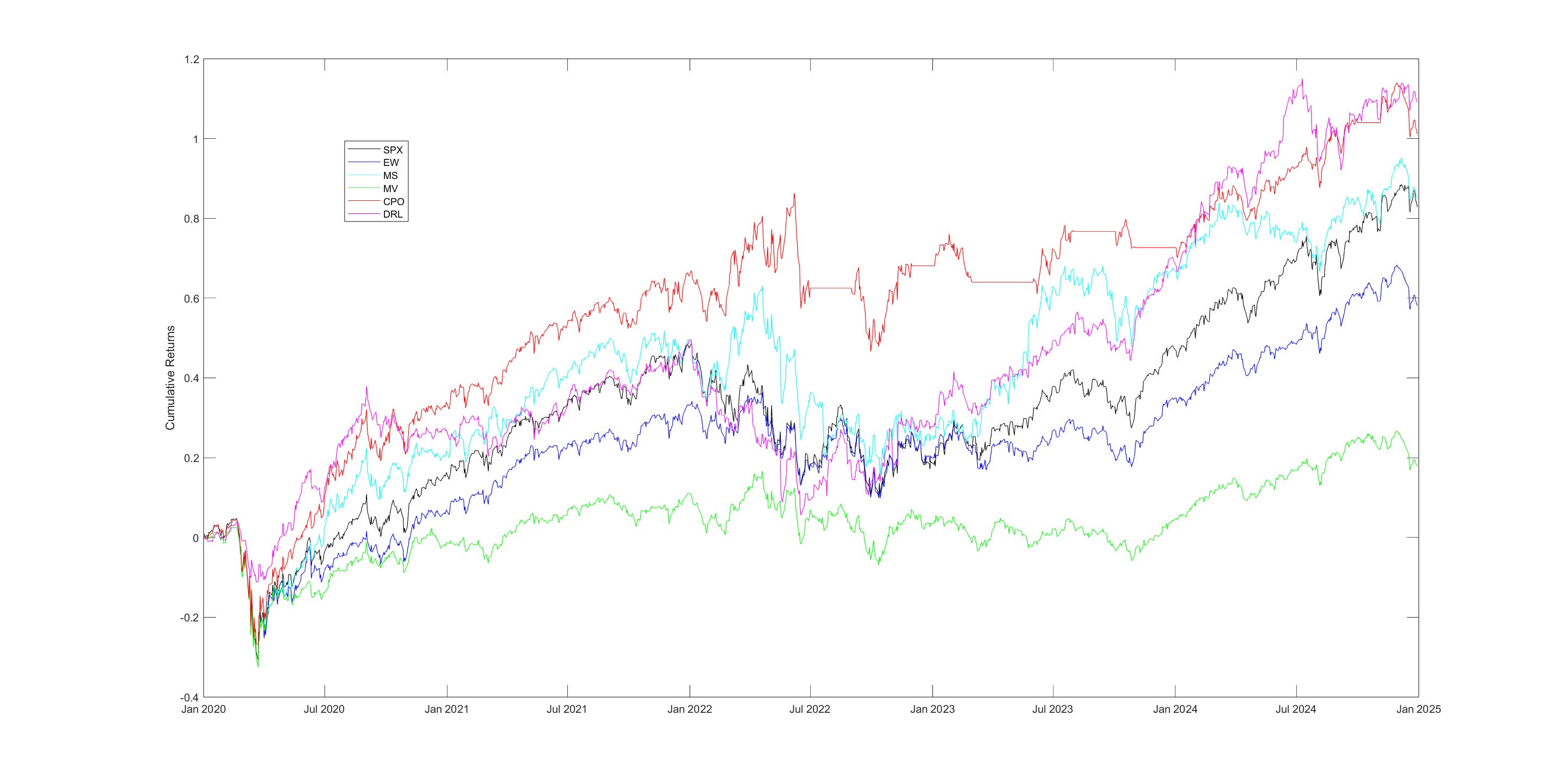
You can see that indeed DRL has the best Sharpe ratio. But here is the caveat: the DRL in Ref.[1] specifies daily rebalancing, which can incur large transaction costs for which our reward function hasn’t accounted, while all other methods except EW are based on monthly rebalancing that incurs far less cost. If we also force DRL to rebalance monthly, the results (in the last column of the table) drop precipitously, and PredictNow.ai's CPO method still performs best. Nevertheless, this is a good illustration of how DRL is supposed to work for portfolio optimization, and we can perhaps improve it using better features and better feature transformation/selection methods, as outlined in the previous blog posts, better network architecture adapted to time-series features, or better hyperparameter optimization.
References:
[1] Sood et. al. (2023). “Deep Reinforcement Learning for Optimal Portfolio Allocation: A Comparative Study with Mean-Variance Optimization"
[2] Levine, S. et. al. (2020). “Offline Reinforcement Learning: Tutorial, Review, and Perspectives on Open Problems”
[3] HuggingFace Deep RL Course
[4] Suarez, J. “Reinforcement Learning Quickstart Guide”
[5] Varatharajan, B. “High Variance in Policy gradients”
[6] Murphy, K. (2024) “Reinforcement Learning: An Overview”
[7] Chan, E. et. al. (2023) “Conditional Portfolio Optimization: Using Machine Learning to Adapt Capital Allocations to Market Regimes”
 | A guest post by
|
 | A guest post by
|
 | A guest post by
|
Great piece to see an application of RL. I’ve always felt RL is difficult to apply in real markets given the vast state space required. Interesting use case here though.